Example Usage

1D interpolation case

Let's interpolate function $f(x)$

\[f(x) = \begin{cases} 0 \, , & 1 \le x \lt 6 \\ 1 \, , & 6 \le x \le 10 \\ -x/5 + 3 \, , & 6 \le x \le 15 \\ 0 \, , & 15 \le x \le 20 \end{cases}\]

by values of the function in nodes $\{1, 2, 3, ..., 20\}$ (case A) and by values of the function and values of its first derivatives in the same nodes (case B). Firstly we'll build a spline using the reproducing kernel RK_H1():

A)

    using NormalHermiteSplines

    x = collect(1.0:1.0:20)       # function nodes
    u = x.*0.0                    # function values in nodes
    for i in 6:10
        u[i] = 1.0
    end
    for i in 11:14
        u[i] = -0.2 * i + 3.0
    end

    # An estimation of the 'scaling parameter' the spline being built with
    ε_estimation = estimate_epsilon(x, RK_H1())

0.7125346243561634

    # Build a differentiable spline by values of function in nodes
    # (a spline built with RK_H0 kernel is a continuous function,
    #  a spline built with RK_H1 kernel is a continuously differentiable function,
    #  a spline built with RK_H2 kernel is a twice continuously differentiable function).
    # Here value of the 'scaling parameter' ε is estimated in the interpolate procedure.
    spline = prepare(x, RK_H1())

    # A value of the 'scaling parameter' the spline was built with.
    ε = get_epsilon(spline)

0.7125346243561634

    # An estimation of the Gram matrix condition number
    cond = estimate_cond(spline)

1.0e7

    # Construct the spline for given 'u' values
    spline = construct(spline, u)

    # An estimation of the interpolation accuracy -
    # number of significant digits in the function value interpolation result.
    significant_digits = estimate_accuracy(spline)

10

    p = collect(1.0:0.2:20)        # evaluation points
    σ = evaluate(spline, p)

    dσ = similar(p)
    for i=1:length(p)
        dσ[i] = evaluate_derivative(spline, p[i])
    end

Evaluate the spline at some points:

    p = [3.1, 8.1, 12.1, 18.1]
    σ = evaluate(spline, p)

4-element Vector{Float64}:
 0.005233851103583653
 1.0029716012459877
 0.5803978696614296
 0.00016170140376470243

Evaluate the spline derivatives at the same evaluation points:

    dσ = similar(p)
    for i=1:length(p)
        dσ[i] = evaluate_derivative(spline, p[i])
    end
    dσ

4-element Vector{Float64}:
  0.05769978169913316
  0.021648276550965222
 -0.1974246697636616
  0.0013127826521445612

Construct spline by different function values in nodes and evaluate new spline at the same evaluation points:

    u2 = 2.0 .* u
    spline = construct(spline, u2)
    σ = evaluate(spline, p)

4-element Vector{Float64}:
 0.010467702207167306
 2.0059432024919754
 1.1607957393228592
 0.00032340280752940487

B)

    using NormalHermiteSplines

    x = collect(1.0:1.0:20)       # function nodes
    u = x.*0.0                    # function values in nodes
    for i in 6:10
        u[i] = 1.0
    end
    for i in 11:14
        u[i] = -0.2 * i + 3.0
    end

    s = x                         # function first derivative nodes
    v = x.*0.0                    # function first derivative values
    for i in 11:14
        v[i] = -0.2
    end

    # Build a differentiable spline by values of function,
    # and values of its first derivatives in nodes
    # (a spline built with RK_H0 kernel is a continuous function,
    #  a spline built with RK_H1 kernel is a continuously differentiable function,
    #  a spline built with RK_H2 kernel is a twice continuously differentiable function).
    # Here value of the 'scaling parameter' ε is estimated in the interpolate procedure.
    spline = interpolate(x, u, s, v, RK_H1())

    # A value of the 'scaling parameter' the spline was built with
    ε = get_epsilon(spline)

1.1092343969889604

    # An estimation of the Gram matrix condition number
    cond = estimate_cond(spline)

1.0e7

    # An estimation of the interpolation accuracy -
    # number of significant digits in the function value interpolation result.
    significant_digits = estimate_accuracy(spline)

11

    p = collect(1.0:0.2:20)      # evaluation points
    σ = evaluate(spline, p)

    dσ = similar(p)
    for i=1:length(p)
        dσ[i] = evaluate_derivative(spline, p[i])
    end

Evaluate the spline at some points:

    p = [3.1, 8.1, 12.1, 18.1]
    σ = evaluate(spline, p)

4-element Vector{Float64}:
 -5.3788085097039584e-12
  0.9999999960755588
  0.5799999979738004
 -3.296918293926865e-12

Evaluate the spline derivatives at the same evaluation points:

    dσ = similar(p)
    for i=1:length(p)
        dσ[i] = evaluate_derivative(spline, p[i])
    end
    dσ

4-element Vector{Float64}:
  1.4839124081558303e-12
 -6.969100085323014e-8
 -0.20000003580236425
  5.95733988455705e-13

C)

Now let's interpolate function $f(x)$ using a spline built with reproducing kernel RK_H0:

    using NormalHermiteSplines

    x = collect(1.0:1.0:20)       # function nodes
    u = x.*0.0                    # function values in nodes
    for i in 6:10
        u[i] = 1.0
    end
    for i in 11:14
        u[i] = -0.2 * i + 3.0
    end

    # Build a continuous spline by values of function in nodes
    # Here value of the 'scaling parameter' ε is estimated in the interpolate procedure.
    spline = interpolate(x, u, RK_H0())

    # A value of the 'scaling parameter' the spline was built with
    ε = get_epsilon(spline)

0.47502308290410894

    # An estimation of the Gram matrix condition number
    cond = estimate_cond(spline)

10000.0

    # An estimation of the interpolation accuracy -
    # number of significant digits in the function value interpolation result.
    significant_digits = estimate_accuracy(spline)

14

    p = collect(1.0:0.2:20)        # evaluation points
    σ = evaluate(spline, p)

Evaluate the spline at some points:

    p = [3.1, 8.1, 12.1, 18.1]
    σ = evaluate(spline, p)

4-element Vector{Float64}:
  1.5445641125352925e-15
  0.9999718738633213
  0.5799851868686876
 -4.200360956850355e-15

This spline is an infinitely differentiable function everywhere excepting the spline nodes. Its derivative does not exist at spline nodes but we can differentiate the spline at other points. Let's evaluate the spline derivatives at the same evaluation points (which do not coincide with the spline nodes):

    dσ = similar(p)
    for i=1:length(p)
        dσ[i] = evaluate_derivative(spline, p[i])
    end
    dσ

4-element Vector{Float64}:
 -1.0224932880036346e-15
 -0.0002500089317770269
 -0.20012979651612287
  2.082761353385413e-15

2D interpolation case

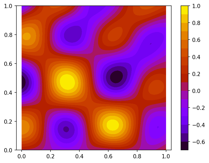
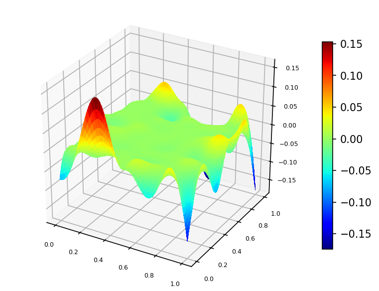
Let's interpolate function $\phi (x,y) = \frac{2}{3}cos(10x)sin(10y) + \frac{1}{3}sin(10xy)$ defined on unit square $\Omega = [0,1]^2$.

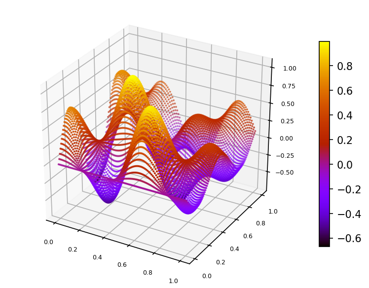
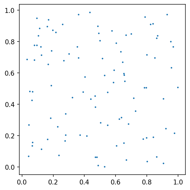
We built a spline using function $\phi$ values sampled on set of 100 pseudo-random nodes uniformly distributed on $\Omega$ (case A).

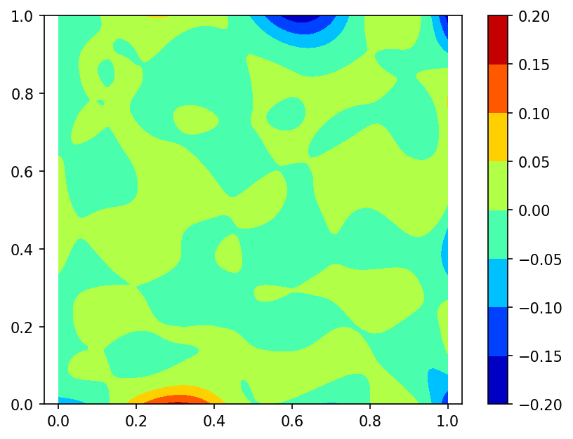
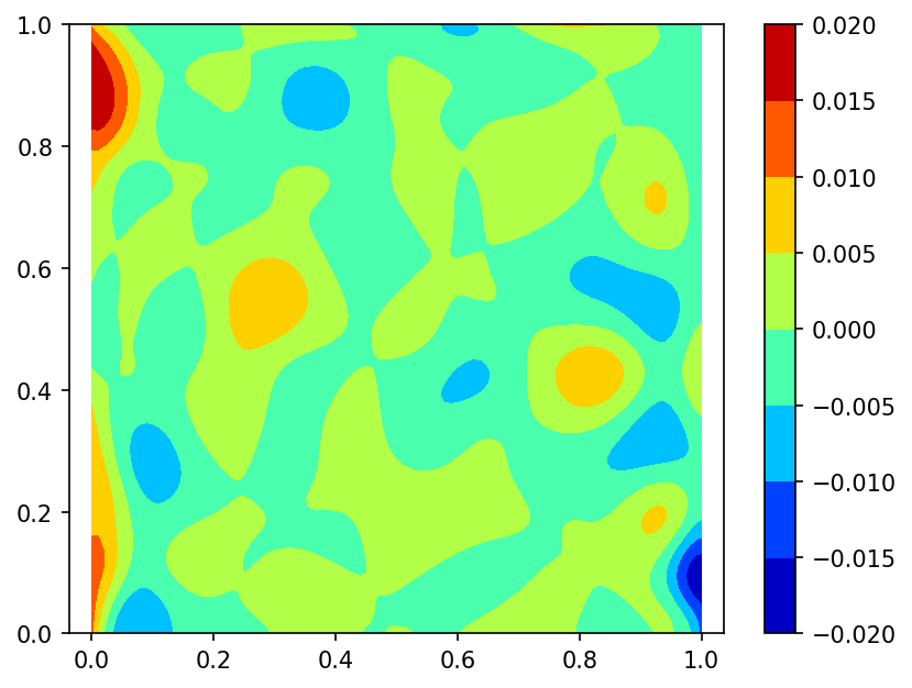
Spline plot                                                                       Approximation error plots

and

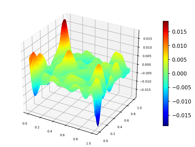
using function $\phi$ values sampled on set of 100 pseudo-random nodes uniformly distributed on $\Omega$ and 80 function $\phi$ gradient values defined at nodes located on the border of domain $\Omega$ (case B):

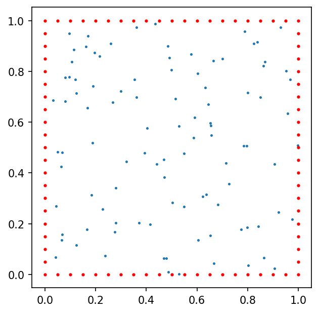
here red dots represent the function $\phi$ gradient nodes.

Spline plot                                                                        Approximation error plots

Following is the code example for case A:

    using Random
    using NormalHermiteSplines

    # generating 100 uniform random nodes
    m = 100
    nodes = Matrix{Float64}(undef, 2, m)
    rng = MersenneTwister(0);
    rnd = rand(rng, Float64, (2, m))
    for i = 1:m
        nodes[1, i] = rnd[1, i]
        nodes[2, i] = rnd[2, i]
    end

    u = Vector{Float64}(undef, m)     # function values at nodes
    for i = 1:m
        x = nodes[1,i]
        y = nodes[2,i]
        u[i] = (2.0*cos(10.0*x)*sin(10.0*y) + sin(10.0*x*y))/3.0
    end

    # creating the uniform Cartesian grid of size 101x101 on [0, 1]x[0, 1]
    t = 100
    x = collect(range(0.0, 1.0; step = 1.0/t))
    y = collect(range(0.0, 1.0; step = 1.0/t))

    t1 = t + 1
    n = t1^2
    grid = Matrix{Float64}(undef, 2, n)
    for i = 1:t1
        for j = 1:t1
            r = (i - 1) * t1 + j
            grid[1, r] = x[i]
            grid[2, r] = y[j]
        end
    end

    f = Vector{Float64}(undef, n)
    for i = 1:n
        x = grid[1,i]
        y = grid[2,i]
        f[i] = (2.0*cos(10.0*x)*sin(10.0*y) + sin(10.0*x*y))/3.0
    end

    # Here spline is constructed with RK_H2 kernel,
    # the value of the 'scaling parameter' ε is estimated
    # in the interpolate procedure.
    rk = RK_H2()
    spline = interpolate(nodes, u, rk)
    #
    # A value of the 'scaling parameter' the spline was built with
    ε = get_epsilon(spline)

3.484398902180334

    # An estimation of the Gram matrix condition number
    cond = estimate_cond(spline)

1.0e10

    # An estimation of the interpolation accuracy -
    # number of significant digits in the function value interpolation result.
    significant_digits = estimate_accuracy(spline)

11

    σ = evaluate(spline, grid)
    # Return the Root Mean Square Error (RMSE) of interpolation
    rmse = sqrt(sum((f .- σ).^2)) / sqrt(length(f))

0.02209299026656501

   # Return the Maximum Absolute Error (MAE) of interpolation
   mae = maximum(abs.(f .- σ))

0.17939052507941705

Value of function $\phi$ at evaluation point $p = [0.5; 0.5]$

    p = [0.5; 0.5]
    x = p[1]
    y = p[2]
    f = (2.0*cos(10.0*x)*sin(10.0*y) + sin(10.0*x*y))/3.0

0.018150344404862222

Value of spline at the evaluation point:

    σ = evaluate_one(spline, p)

0.017166894615229467

Difference of function $\phi$ and spline values at the evaluation point:

    diff = f - σ

0.0009834497896327558

Gradient of function $\phi$ at the evaluation point

    g1 = (10.0*y*cos(10.0*x*y) - 20.0*sin(10.0*x)*sin(10.0*y))/3.0
    g2 = (20.0*cos(10.0*x)*cos(10.0*y) + 10.0*x*cos(10.0*x*y))/3.0
    f_grad = [g1; g2]

2-element Vector{Float64}:
 -7.465477789499732
 -0.7988111228330643

Gradient of spline at the evaluation point

    σ_grad = evaluate_gradient(spline, p)

2-element Vector{Float64}:
 -7.4815682885317285
 -0.8051369242783533

Norm of difference of function $\phi$ and spline gradient values at the evaluation point:

    diff_grad = sqrt(sum((f_grad .- σ_grad).^2))

0.017289300825189386

Corresponding code example for case B:

    using Random
    using NormalHermiteSplines

    function get_2D_border_nodes(m::Int)
        mat0 = [0.0 0.0; 0.0 1.0; 1.0 0.0; 1.0 1.0]'
        if m < 1
            return mat0
        end
        m1 = m + 1
        p = collect(range(1.0/m1, (1.0 - 1.0/m1); step = 1.0/m1))
        ms = m * 4
        mat = Matrix{Float64}(undef, 2, ms)
        for i = 1:m
            mat[1,i] = 0.0
            mat[2,i] = p[i]
        end
        for i = (m+1):(2*m)
            mat[1,i] = 1.0
            mat[2,i] = p[i-m]
        end
        for i = (2*m+1):(3*m)
            mat[1,i] = p[i-2*m]
            mat[2,i] = 0.0
        end
        for i = (3*m+1):(4*m)
            mat[1,i] = p[i-3*m]
            mat[2,i] = 1.0
        end
        w = hcat(mat0, mat)
        return w
    end

    # generating 100 uniform random nodes
    m = 100
    nodes = Matrix{Float64}(undef, 2, m)
    rng = MersenneTwister(0);
    rnd = rand(rng, Float64, (2, m))
    for i = 1:m
        nodes[1, i] = rnd[1, i]
        nodes[2, i] = rnd[2, i]
    end

    u = Vector{Float64}(undef, m)     # function values at nodes
    for i = 1:m
        x = nodes[1,i]
        y = nodes[2,i]
        u[i] = (2.0*cos(10.0*x)*sin(10.0*y) + sin(10.0*x*y))/3.0
    end

    bnodes = get_2D_border_nodes(19)   # 80 border nodes
    bn_1 = size(bnodes, 2)
    d_nodes = Matrix{Float64}(undef, 2, bn_1)
    es = Matrix{Float64}(undef, 2, bn_1)
    du = Vector{Float64}(undef, bn_1)
    grad = [0.0; 0.0]
    for i = 1:bn_1
        x = bnodes[1,i]
        y = bnodes[2,i]
        d_nodes[1,i] = x
        d_nodes[2,i] = y
        grad[1] = (10.0*y*cos(10.0*x*y) - 20.0*sin(10.0*x)*sin(10.0*y))/3.0
        grad[2] = (20.0*cos(10.0*x)*cos(10.0*y) + 10.0*x*cos(10.0*x*y))/3.0
        es[1,i] = grad[1]            # no need to normalize 'es' vectors
        es[2,i] = grad[2]
        du[i] = sqrt(grad[1]^2 + grad[2]^2)
    end

    # creating the uniform Cartesian grid of size 101x101 on [0, 1]x[0, 1]
    t = 100
    x = collect(range(0.0, 1.0; step = 1.0/t))
    y = collect(range(0.0, 1.0; step = 1.0/t))

    t1 = t + 1
    n = t1^2
    grid = Matrix{Float64}(undef, 2, n)
    for i = 1:t1
        for j = 1:t1
            r = (i - 1) * t1 + j
            grid[1, r] = x[i]
            grid[2, r] = y[j]
        end
    end

    f = Vector{Float64}(undef, n)
    for i = 1:n
        x = grid[1,i]
        y = grid[2,i]
        f[i] = (2.0*cos(10.0*x)*sin(10.0*y) + sin(10.0*x*y))/3.0
    end

    # Here spline is constructed with RK_H2 kernel,
    # the 'scaling parameter' ε is defined explicitly.
    rk = RK_H2(1.0)
    spline = interpolate(nodes, u, d_nodes, es, du, rk)
    #
    # A value of the 'scaling parameter' the spline was built with
    ε = get_epsilon(spline)

1.0

    # An estimation of the Gram matrix condition number
    cond = estimate_cond(spline)

1.0e13

    # An estimation of the interpolation accuracy -
    # number of significant digits in the function value interpolation result.
    significant_digits = estimate_accuracy(spline)

9

    σ = evaluate(spline, grid)
    # Return the Root Mean Square Error (RMSE) of interpolation
    rmse = sqrt(sum((f .- σ).^2)) / sqrt(length(f))

0.0033315866550400375

   # Return the Maximum Absolute Error (MAE) of interpolation
   mae = maximum(abs.(f .- σ))

0.01913080857367011

Value of function $\phi$ at evaluation point $p = [0.5; 0.5]$

    p = [0.5; 0.5]
    x = p[1]
    y = p[2]
    f = (2.0*cos(10.0*x)*sin(10.0*y) + sin(10.0*x*y))/3.0

0.018150344404862222

Value of spline at the evaluation point:

    σ = evaluate_one(spline, p)

0.01733527009446334

Difference of function $\phi$ and spline values at the evaluation point:

    diff = f - σ

0.0008150743103988826

Gradient of function $\phi$ at the evaluation point

    g1 = (10.0*y*cos(10.0*x*y) - 20.0*sin(10.0*x)*sin(10.0*y))/3.0
    g2 = (20.0*cos(10.0*x)*cos(10.0*y) + 10.0*x*cos(10.0*x*y))/3.0
    f_grad = [g1; g2]

2-element Vector{Float64}:
 -7.465477789499732
 -0.7988111228330643

Gradient of spline at the evaluation point

    σ_grad = evaluate_gradient(spline, p)

2-element Vector{Float64}:
 -7.48378137008649
 -0.7997070273895588

Norm of difference of function $\phi$ and spline gradient values at the evaluation point:

    diff_grad = sqrt(sum((f_grad .- σ_grad).^2))

0.018325493370446602

Q & A

Q1. Question: The call

spline = interpolate(x, u, RK_H2())

cause the following error: PosDefException: matrix is not positive definite; Cholesky factorization failed. What is a reason of the error and how to resolve it?

A1. Answer: Creating a Bessel potential space reproducing kernel object with omitted scaling parameter ε means that this parameter will be estimated during interpolating procedure execution. It might happen that estimated value of the ε is too small and corresponding Gram matrix of the system of linear equations which defines the normal spline coefficients is a very ill-conditioned one and it lost its positive definiteness property because of floating-point rounding errors.

There are two ways to fix it.

• We can get the estimated value of the parameter ε by calling get_epsilon function:

ε = get_epsilon(spline)

then we can call the interpolate function with a larger value of this parameter:

larger_ε = 5.0*ε
spline = interpolate(x, u, RK_H2(larger_ε))

• We may change the precision of floating point calculations. Namely, it is possible to use Julia standard BigFloat numbers or Double64 - extended precision float type from the package DoubleFloats:

using DoubleFloats

x = Double64.(x)
u = Double64.(u)
ε = Double64(1.0)
spline = interpolate(x, u, RK_H2(ε))

This answer also applies to reproducing kernel object of type RK_H0 or RK_H1.

Q2. Question: The following calls

spline = interpolate(x, u, RK_H2())
σ = evaluate(spline, p)

produce the output which is not quite satisfactoty. Is it possible to improve the quality of interpolation?

A2. Answer: Creating a Bessel potential space reproducing kernel object with omitted scaling parameter ε means that this parameter will be estimated during interpolating procedure execution. It might happen that estimated value of the ε is too large and it is possible to use a smaller value of ε which can lead to a better quality of interpolation.

• We can get the value of scaling parameter ε by calling get_epsilon function

ε = get_epsilon(spline)

and get an estimation of the problem's Gram matrix condition number by calling estimate_cond function as well as an estimation of the number of the significant digits in the interpolation result by calling estimate_accuracy function:

cond = estimate_cond(spline)
significant_digits = estimate_accuracy(spline)

In a case when estimated number of the significant digits is bigger than 10 and estimated condition number is not very large, i.e. it is less than $10^{12}$, we may attempt to build a better interpolating spline by calling interpolate function with a smaller value of the scaling parameter:

e_smaller = ε/2.0 
spline = interpolate(x, u, RK_H2(e_smaller))
cond = estimate_cond(spline)
significant_digits = estimate_accuracy(spline)
σ = evaluate(spline, p)

Taking into account new cond and significant_digits values we decide of making further correction of the scaling parameter.

For further information, see Selecting a good value of the scaling parameter.